System Design: Sharding and Data Partitioning

12 July 2026 - 22 mins read time
Tags: System Design Distributed Systems Databases Sharding Scalability

At some point every growing system hits the same wall: a single database can no longer hold the data — or serve the load — fast enough. The usual reflex is to buy a bigger machine. That works until it doesn’t, because vertical scaling has a hard ceiling and a single expensive point of failure. Sharding is the technique that lets you grow sideways instead: break the data into smaller pieces and spread them across many nodes.

This post walks through sharding from first principles: what it is, why it enables horizontal scale, the two concepts that make or break it (sharding keys and hot partitions), and the concrete strategies used in production — from naive range splits to consistent hashing and shuffle sharding.

Defining sharding

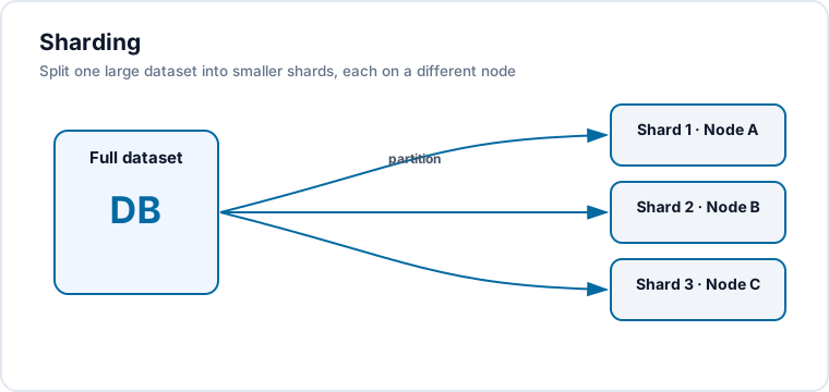
Sharding (also called partitioning) is a distributed-systems technique that splits a large dataset into smaller chunks called shards (or partitions). Each shard holds only a slice of the whole, which makes it possible to handle massive volumes of data more efficiently, more securely, and with higher availability. It becomes essential exactly when the data grows past the point where a single server, database, or workload can serve it performantly.

The idea isn’t limited to databases. Although that’s its most common use, the same partitioning principle applies to distributing load across microservices, to distributed caches, and even to segmenting network traffic.

In a database context, each shard is a subset of the original base that can live on a different server or node. That division distributes the work, eliminates bottlenecks, and removes the single points of failure that appear when everything is centralised. It’s also what makes horizontal scalability possible: as data grows, you add new servers to host additional shards.

The trade-off is real, though. Sharding introduces maintenance and rebalancing complexity, plus the ongoing challenge of keeping data consistent across partitions as scale increases.

Sharding splits one large dataset into smaller shards, each living on a different node.

Sharding topologies

There isn’t just one way to shard. Different topologies suit different needs; thinking about the concept broadly, several distinct approaches exist to distribute load and gain performance and resilience.

Sharding for data segregation is the best-known form. The goal is to separate different sets of data into distinct shards — tables or database instances routed by some criterion. It’s common in systems that must isolate data types for security, compliance, or simply for easier management and performance. In a multi-tenant application, for example, each major customer’s data can be segregated into its own shard: this reinforces security by preventing one customer from accessing another’s data, and it lets you tailor each shard’s infrastructure to that customer’s specific needs. Another recurring case is separating sensitive from non-sensitive data — confidential or regulated information can sit in shards with stronger security and auditing, while less critical data lives in lighter, cheaper shards.

Sharding for computational segregation shifts the focus from the data to the compute load. Instead of distributing records, the idea is to isolate intensive operations onto dedicated shards. In systems that run heavy tasks — real-time calculations, large-volume processing, machine-learning algorithms — segregating that processing onto specific shards keeps lighter operations from being starved of resources, so the system as a whole stays predictable. This topology also helps when different operations need different hardware: I/O-intensive shards can use fast disks and more bandwidth, while compute-heavy shards can be provisioned with more CPU cores.

Scalability and performance

Sharding matters in distributed systems precisely because of the need to handle large data volumes and to scale horizontally. The database is frequently the most critical point of scale, and sharding acts right at that bottleneck.

By dividing data across several shards hosted on different servers, you can add capacity without restructuring the entire base, expanding infrastructure as demand grows. That horizontal elasticity is essential for systems that must grow continuously without sacrificing performance or integrity.

With the data fragmented, read and write operations also spread across distinct resources. This reduces the load on any individual server, improves response times, and avoids bottlenecks — sustaining consistent performance even under high load.

There’s an availability gain too: if the node hosting one shard fails, the remaining shards stay active, letting the system operate with reduced functionality instead of a total outage — a crucial form of resilience in production environments.

Sharding keys and hot partitions

Before looking at concrete implementations, two complementary concepts sit at the centre of partitioning theory: the sharding key and the phenomenon of hot partitions.

Sharding keys

The first question when planning a partitioning scheme is: “partition based on what?” Choosing the dimension to cut on is the most important decision — it comes before any technology choice. That cutting criterion is the sharding key.

The sharding key (or partition key) is the attribute that determines how, and into which partition, each piece of data is stored. A good choice must guarantee balanced distribution, which usually demands high cardinality — a large number of unique values. Ideally the key should also align with fields frequently used in queries, such as dates, identifiers, or categories.

Common sharding keys include the initials of a customer identifier, an entity ID, the hash of some value, or specific categories. In financial systems it’s common to separate individuals from companies; banks may partition by branch ranges; sales and logistics systems often split by date ranges; and multi-tenant systems frequently use the hash of the tenant identifier. The right strategy depends on context and on the characteristics of the system.

Hot partitions

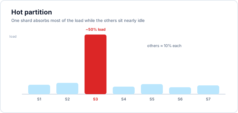
Hot partitions are the problem that arises from poor distribution of data and load across partitions. It happens when one or a few partitions receive a disproportionately high share of the load relative to the rest, degrading performance.

Imagine a multi-tenant system with 300 customers spread across 10 partitions. In the ideal case each partition holds about 30 customers, or ~10% of usage. But suppose three of those customers account for 50% of all usage and — by an unlucky hash — land on the same partition. That single partition now carries more than half the load, while the other nine sit nearly idle. That’s a hot partition.

Because the distribution is defined by mathematical operations on the key — not by the real size or usage pattern of the data — this imbalance can appear naturally. Overloaded partitions cause slowness and, in extreme cases, failures, while underused ones waste resources. Mitigations include using more random partition keys, pre-partitioning based on known usage patterns, isolating specific sharding keys onto dedicated partitions, and applying intelligent caching to relieve the most-accessed partitions.

A hot partition: one shard absorbs a disproportionate share of the load while the others sit nearly idle.

Sharding strategies

There are many ways to apply sharding. The sections below walk through the most common ones, from the simplest (and most flawed) to the techniques used in large-scale production systems.

By ranges of initials

A simple — not very effective, but instructive — strategy distributes users, customers, or tenants by the initials of an identifier. You define letter ranges per shard: say A–E on one shard, F–J on another, and so on through W–Z.

Easy as it is to understand, this model exposes exactly the problem sharding is meant to avoid: hot partitions. When usage is uneven across the ranges, imbalance follows. With name initials, it’s reasonable to assume there are far more people whose names start with A, B, or C than with W, Y, or Z. So the A–E partition becomes a hot partition while W–Z stays almost idle — a stark performance imbalance. The lesson: choose a sharding key that promotes balanced distribution.

By ranges of identifiers

Another common approach divides data by continuous ranges of the sharding key’s values. Being sequential, it demands more governance, because it can produce an “overflow” effect: some shards fill up while others stay empty or underused.

Each shard contains a specific band of values, and queries are routed to the corresponding shard. It works well when data has a natural order and queries tend to involve ranges. Picture a base of 10,000 sequentially created users, split across 3 shards by identifier bands, with room reserved for new sign-ups. Taken literally, the sequential nature can leave you with two full shards and one nearly empty, holding capacity for growth.

The risk is load imbalance: if values don’t distribute evenly, some shards hit their limit while others idle. When using identifier ranges, it’s mandatory to monitor and rebalance the distribution as the system grows.

By date ranges and storage tiers

Sequential attributes also enable sharding by time intervals. In a hypothetical sales system, you could partition by date ranges — for example, one base per year, grouping all transactions from that period.

This model pairs naturally with a very common companion strategy: storage tiers. The idea is to organise data into layers with different cost and performance profiles. The current and previous years could sit in a hot tier, on expensive, fast storage; years accessed with moderate frequency move to an intermediate warm tier; and very old, rarely queried data goes to a cold tier that’s cheaper and slower. Combining date partitioning with storage tiers delivers efficient distribution and cost/performance optimisation, matching resources to how often — and how important — the data is over time.

By hashing

In hash-based sharding, you apply a hash function to the sharding key to decide where the data is stored, or where the client is routed. The function turns the key value into a hash, which is then mapped to one of the available shards via a modulo (mod) operation — the remainder of a division.

For example, if the hash is 15 and there are 3 shards, 15 % 3 = 0, pointing to shard 0. If the hash is 10, 10 % 3 = 1, sending the record to shard 1.

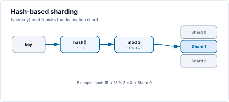
Hash-based sharding: a hash of the key, reduced modulo the shard count, decides the destination shard.

Consider a multi-tenant system where the tenant identifier is the sharding key. To pick each customer’s shard, you hash the identifier (say with SHA-256), turn the hash into an integer, and take the modulo by the number of shards; the remainder is the destination shard:

const numShards = 3

// hashTenant returns a stable integer hash for a tenant identifier.
func hashTenant(tenant string) uint64 {
	sum := sha256.Sum256([]byte(strings.ToLower(tenant)))
	return binary.BigEndian.Uint64(sum[:8])
}

// getShardByTenant maps a tenant to one of numShards partitions.
func getShardByTenant(tenant string) uint64 {
	return hashTenant(tenant) % numShards
}

This helps avoid hot partitions, since a good hash function tends to distribute data uniformly, and the modulo itself is cheap — efficient even at large scale.

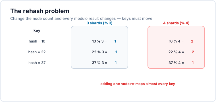
The scheme is simple, intuitive, and works well — until the number of servers changes. If a server fails or a new one is added, the keys must be redistributed, because the modulo result changes: hash % 3 and hash % 4 send the same key to different shards. In other words, whenever the server count varies, you lose the distribution references.

For stateless resources like application servers, that redistribution is trivial. For state that’s easily rebuilt, like caches, the impact is small. But for partitions holding persistent data, changing the server count becomes a serious problem — you can lose the routing to the original storage and generate immediate inconsistencies, forcing an expensive redistribution right after any horizontal scaling event. To mitigate this when nodes change often, you reach for consistent hashing.

The rehash problem: changing the server count changes every modulo result, so keys lose their mapping and must be redistributed.

Choosing the hash algorithm

The choice of hash algorithm is a fine-tuning point that can completely change the resulting distribution. After choosing the sharding key well, it’s worth comparatively testing several algorithms over a sample of keys to see which gives the best spread. Depending on the algorithm, data lands more or less evenly across shards, directly affecting performance and resilience.

You might, for instance, compare SHA-256, SHA-512, MD5, FNV-1a, and a naive sum-of-character-codes function over the same set of tenants, counting how many land in each shard. The counts vary noticeably between algorithms — some balance well, others concentrate entries on particular shards. One caveat: a result like that is only valid for that specific set of sharding keys. With different values the outcome can be completely different; the experiment only illustrates how much the algorithm choice matters.

Distribution with MurmurHash

MurmurHash (or just Murmur) is a fast, efficient, non-cryptographic hash function widely used to generate identifiers from strings and other data. It converts data into integers, handling ranges natively, which makes it especially useful for data distribution and consistent hashing. It excels at avoiding hot partitions because it spreads hash values close to uniformly.

Applying MurmurHash to a string used as a sharding key produces a numeric value directly — a 32- or 64-bit integer depending on the version — with no extra conversions. Its simplicity and low computational cost make it ideal for systems that must process large volumes quickly:

import "github.com/spaolacci/murmur3"

// getShardMurmur routes a tenant to a shard using a 32-bit Murmur hash.
func getShardMurmur(tenant string, shards uint32) uint32 {
	return murmur3.Sum32([]byte(tenant)) % shards
}

Run over a set of tenants, the resulting per-shard counts come out very close to each other — evidence of MurmurHash’s tendency toward uniform distribution.

Consistent hashing

Consistent hashing is a sharding technique that shines in distributed systems where adding or removing servers is routine. Unlike plain hashing — where changing the shard count can force redistributing almost all the data — consistent hashing minimises how much data moves. Redistribution still happens, but on a far smaller scale.

Visually, consistent hashing is cyclic: the central structure is a ring, the hash ring. A key is allocated to a node by falling into an interval of values on the ring, not by an exact hash match. So when you change the number of nodes, results shift very little, cutting the redistribution needed.

Back to the multi-tenant system: imagine a circle representing every possible hash value. Both the server nodes and the tenants are mapped onto points on that circle using the same function. A tenant’s data lives on the first server found clockwise from the tenant’s point; if the value passes the end, it “wraps around” back to marker 0 on the ring. When you add a new node, only the data between it and the next node clockwise needs to move; everything else stays put. When you remove a node, its data passes to the next node clockwise — minimal movement, preserved integrity.

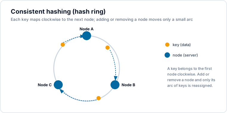
The hash ring: nodes and keys map onto a circle, and each key belongs to the first node clockwise — so adding or removing a node moves only a small arc.

A minimal ring, with binary search to find the owning node, looks like this:

type HashRing struct {
	replicas int               // virtual nodes per physical node
	keys     []uint32          // sorted hash values
	ring     map[uint32]string // hash -> node name
}

func (r *HashRing) AddNode(node string) {
	for i := 0; i < r.replicas; i++ {
		h := murmur3.Sum32([]byte(fmt.Sprintf("%s-%d", node, i)))
		r.keys = append(r.keys, h)
		r.ring[h] = node
	}
	sort.Slice(r.keys, func(i, j int) bool { return r.keys[i] < r.keys[j] })
}

func (r *HashRing) GetNode(key string) string {
	if len(r.keys) == 0 {
		return ""
	}
	h := murmur3.Sum32([]byte(key))
	// first virtual node clockwise from the key's position
	idx := sort.Search(len(r.keys), func(i int) bool { return r.keys[i] >= h })
	if idx == len(r.keys) {
		idx = 0 // wrap around the ring
	}
	return r.ring[r.keys[idx]]
}

Adding virtual replicas per physical node (the replicas field above) smooths the distribution, so no single node owns an oversized arc of the ring. If you distribute tenants, then remove one shard and add another, only a handful of tenants change shards on each change — the rest stay where they were. That small-movement property is exactly what makes consistent hashing attractive. It also accepts many hash algorithms, so it’s worth benchmarking the balance (as above) to find the best spread for your sample of keys.

Hashing with a key-management service

An alternative treats partition distribution and lookup as a registry concern, which requires extra architecture. The appeal of hashing is that the calculation is very cheap; the pain shows up in redistributions, which can become extremely costly.

Picture an architecture where the hash is computed only at the moment a new sharding key is created, and subsequent lookups go through a dedicated API that exposes those distribution keys over some protocol. This design needs a smart balancing/routing component to forward each request to its correct shard. Despite the greater engineering effort, it offers more manual, controlled management of how customers map to partitions. It lets you isolate customers who cause hot partitions, placing them on segregated shards with dedicated infrastructure so that very intensive users don’t affect overall performance. Because it’s more manual, it also opens the door to combining other design techniques — caching, load balancing, and replication.

Advanced isolation with shuffle sharding

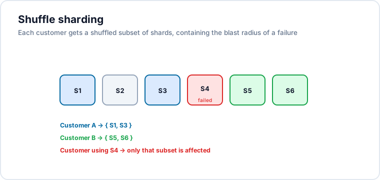
Shuffle sharding is an advanced technique that combines traditional sharding with distributed replication. The idea is to create shuffled subsets of shards for each customer, operation, or partition, drastically reducing the blast radius of a failure. By saving a customer’s data on more than one shard, you isolate failures, load spikes, and malicious behaviour to a minimal group of resources — preventing a single customer from taking down the whole infrastructure, or every customer on one shard.

The model works as a hybrid of replication and sharding. Each operation is routed to a primary shard (the golden source of that customer’s data) and also written to one or more secondary shards chosen by the shuffling algorithm, which defines the customer’s “virtual shuffle-shard.” Consistency comes in two modes: strong consistency, where data is only confirmed after a successful write to N shards in the set, guaranteeing immediate durability; and eventual consistency, where the secondary replicas update asynchronously, favouring low latency and high throughput.

The strategy balances resilience, logical isolation, and scalability. Because each customer writes to multiple shuffled shards, any failure is restricted to the shards that customer uses, not the entire cluster. When a shard fails, its fallbacks take over as primary, redirecting that partition’s customers to a fallback shard with their complete (or nearly complete) data. Overall, the system tolerates more partial failures, because the redundancy between primaries and secondaries sustains reads and writes even during incidents.

Shuffle sharding: each customer is assigned a shuffled subset of shards, so a failure is contained to that subset instead of the whole cluster.

Key takeaways

Sharding is horizontal scale for data. When one machine can’t hold the volume or serve the load, you split the dataset across nodes instead of buying a bigger box — trading a single point of failure for distributed capacity, at the cost of rebalancing and consistency complexity.
The sharding key is the decision that matters most. Pick it before any technology. Aim for high cardinality and alignment with your query patterns, or you’ll design imbalance in from day one.
Hot partitions are the failure mode to watch. Uneven load — not uneven data size — is what degrades a sharded system. Random keys, pre-partitioning, isolation, and caching are your defences.
Plain hash % N breaks when N changes. It’s simple and even, but every scaling event reshuffles almost everything. Fine for stateless nodes and caches; dangerous for persistent data.
Consistent hashing minimises movement. A hash ring with virtual nodes keeps redistribution proportional to the change, which is why it underpins so many distributed caches and datastores.
Shuffle sharding shrinks the blast radius. For multi-tenant systems, shuffled subsets per customer turn a cluster-wide outage into a contained, per-customer one.