System Design: Performance, Capacity, and Scalability
Three topics show up together in almost every System Design conversation: performance, capacity, and scalability. They’re distinct enough to each deserve their own book, but they’re also inseparable — performance defines the limits capacity has to plan around, and scalability is how you move those limits when demand outgrows them. This post treats them as one system, and ends with concrete formulas you can use to right-size infrastructure.
Defining performance
Performance is, in short, a measure of how fast and efficient a system or algorithm is at processing a single transaction — whether in isolation or in the middle of a large volume of concurrent operations. It’s the facet the end user feels most directly, even though it hides a lot of engineering complexity underneath.
Performance always has to be read against the system’s functional and non-functional requirements. A real-time processing service carries very different expectations from a long-term archival system. There’s no “good” number in a vacuum — context is everything.
Performance metrics
To understand how a system behaves under different conditions — load spikes, component failures, shifts in usage patterns — you need continuous monitoring of key indicators. Watching those metrics sequentially, across many periods, feeds decisions about design, maintenance, operation, benchmark comparisons, and where to invest in improvements.
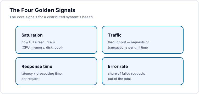
Some metrics are practically universal; others emerge from specific business needs. This post focuses on the universal baseline: the Four Golden Signals, popularised by Google in the Site Reliability Engineering book. Those four signals — saturation, traffic, response time, and error rate — are the core of understanding a distributed system’s health. Here we look at them through a performance lens rather than an observability one.
Utilisation and saturation
Utilisation tells you how much of an available resource is in use. When that rate approaches the maximum possible or expected, the resource is saturated. Saturation can hit CPU, memory, disk, or even a network connection pool — and tracking it helps you anticipate performance problems and know when to scale.
CPU-, memory-, disk-, and network-intensive algorithms are especially sensitive to both optimisation and degradation. Measuring saturation answers questions like “above what CPU percentage does my response time start to suffer?” or “at what disk I/O does my database begin degrading queries?” Being able to answer those clearly is a sign of team maturity.
Utilisation is the ratio of consumed to available resource, times 100:
utilisation% = consumed / available × 100
             = 1 GB / 2 GB × 100 = 50%
One important caveat: a resource can start degrading performance before it ever reaches 100% utilisation.
Throughput (traffic)
Throughput describes how many operations a system completes in a given time window — requests per second, sales per minute, files per day, events per month. In web applications it’s usually counted as HTTP requests received and answered.
You get it by dividing units of work by time. A system that handled 6,000 requests in the last minute has a throughput of 6000 / 60 = 100 rps. Expressing it this way tells you how far the system can go before it starts hurting response time and error rate — and it’s the basis for triggering dynamic scaling.
Response time
Response time is the total interval between sending a request and receiving the answer. It’s the sum of latency (the network round trip) and processing time (the work the server does once the request arrives). From the user’s point of view, it’s the time between taking an action and seeing the result. In a scalable system, this value ideally should not grow significantly as load increases.
Latency reflects network delay — shaped by physical distance, the transmission medium, and intermediate devices like routers. Processing time is what the server spends handling the request after receiving it. Measured from the client, response time is simply the response timestamp minus the request timestamp. Each component can be observed independently and at different points in the flow — granularity that’s invaluable in troubleshooting, because it pinpoints exactly where the degradation happened.
Error rate
The error rate is the percentage of requests that fail relative to the total processed. Combined with response time and throughput, it supports strong conclusions about system behaviour. A well-designed system should hold or reduce its error rate even as load grows.
The calculation is direct — errors divided by total attempts, times 100:
errorRate% = errors / total × 100
           = 50 / 1000 × 100 = 5%
Tracking it over time surfaces trends, quantifies the impact of changes, and prioritises what needs fixing — especially in production, where stability is critical.
Using percentiles
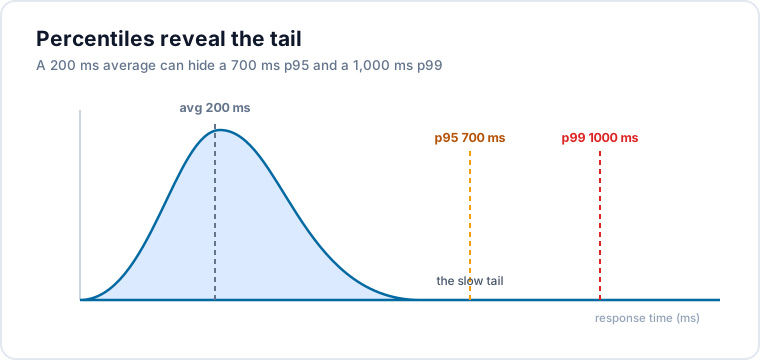
Percentiles split an ordered dataset into a hundred equal parts and give a far richer view than the average alone. In response-time, query-execution, and resource-usage analysis, they reveal the outliers and spikes that averages tend to hide.
A percentile is the value below which a given share of the data falls. A p90 of 800 ms means 90% of responses are faster than that. High percentiles like p95 and p99 are excellent for catching abnormal, extreme behaviour that hurts user experience.
Consider a scenario where the average response is 200 ms — seemingly excellent. Look at the percentiles, though, and the p95 is 700 ms while the p99 reaches 1,000 ms. So although most requests are fast, a meaningful slice of responses is far slower than the average suggests. Evaluating those outliers is essential for planning capacity and finding bottlenecks — which is exactly why “averages hide, percentiles reveal” is a monitoring mantra.
Defining capacity
Capacity is the maximum amount of work a system can receive and process effectively over a given period. It’s how you discover the system’s current limit across CPU, memory, storage, network — and the performance of the algorithms themselves. Over short, medium, and long horizons, monitoring resources and dependencies matters as much as monitoring performance.
The concept is central to architecture and infrastructure planning. It spans both the ability to process data and transactions (tied to compute power and efficiency) and the ability to support many concurrent users without degrading, adapting to rising load to keep the experience constant. Working on capacity isn’t just sizing resources — it also involves monitoring, observability, performance management, automation, and scalability.
Capacity bottlenecks
Bottlenecks are points where performance or capacity is limited by a component that can’t keep up with the load. They can appear in hardware, software, or network architecture. A common mistake — even among experienced engineers — is to associate bottlenecks only with infrastructure, when in practice poorly optimised code, inefficient algorithms, and concurrency problems (deadlocks, excessive locking) are often even harder limiters to overcome.
A design that doesn’t distribute load well creates bottlenecks on its own — for example, a central processing point that should have been split up. In essence, a bottleneck shows up when demand exceeds capacity. Identifying and resolving them is the key to optimising performance and scalability, and it usually takes detailed monitoring, load testing, and fine-tuning. One important detail: resolving one bottleneck lets the load flow onward and can reveal a new bottleneck in the next component. It’s a dynamic, continuous process.
Backpressure
Backpressure borrows its name from physical engineering — specifically fluid dynamics — where it describes resistance opposing the flow of a fluid: obstructions or tight bends create counter-pressure through friction loss and pressure drop.
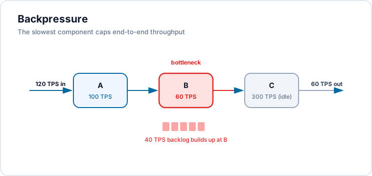
In software, backpressure happens when a component receives more data or requests than it can process, driving up response time, causing failures, and even losing data. Picture a transaction that flows through services A, B, and C, which handle 100, 60, and 300 TPS respectively. At 90 TPS, all three absorb the flow without trouble.
At 100 TPS, though, service B — capped at 60 — accumulates 40 transactions per second of backlog. Push it harder, to 120 TPS injected, and the end-to-end bottleneck settles at 60 TPS: 50% degradation between input and output. The most performant component in the flow (C, at 300 TPS) sits permanently idle, held back by what comes before it. As the maxim goes, “a chain is only as strong as its weakest link” — a system’s throughput and capacity are always constrained by its most degraded component.
Cost per transaction
Evaluating cost per transaction is a way to measure the efficiency and value-for-money of the capacity you’ve allocated. It’s a financial metric that matters especially in public clouds, where every resource shows up on the bill. Normally you count only end-user requests, without multiplying by the internal subsystems and microservices that are transparent to the user.
The calculation divides total operating cost by total transactions in the same period. In systems with variable demand this value shifts over time — which is why the peaks matter. Generally, a lower cost per transaction indicates greater efficiency and better use of resources.
Defining scalability
Scalability is a system’s ability to grow and absorb increasing load without compromising quality, performance, or efficiency — whether that’s more users, transactions, data, or resources. It’s a critical attribute for systems that expect growth, and especially important in the cloud, where demands change quickly.
In Release It!, Michael T. Nygard frames scalability two ways: how throughput varies with demand (relating requests-per-second to response time), and the modes of scaling a system offers. This post adopts the second: the ability to add or remove compute capacity. A useful analogy is an air conditioner set to 20 °C — when the room warms up it ramps power up; when it cools it ramps down, always working to stabilise the target. Scalable systems do the same with their resources.
Why it matters in modern systems
Scalability lets systems adapt quickly to shifts in traffic and demand, holding consistent performance under any load. In dynamic businesses, scaling on demand is what guarantees continuity, operational efficiency, and a satisfying user experience even during peaks.
There’s an economic upside too: scalable systems use resources more efficiently, paying only for what’s used and cutting waste. They also make it easier to evolve the product and add features without a complete overhaul of infrastructure you’ve already designed.
Vertical vs horizontal scalability
There are two broad types of scaling. To illustrate them, imagine a bus company whose mission is to carry passengers from point A to point B. The initial fleet handled about 100 passengers per departure, but growing demand started producing queues, delays, and complaints. Two strategies solve it.
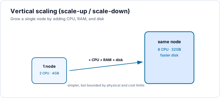
Vertical scalability would swap part of the fleet for double-decker buses, doubling each vehicle’s capacity. That’s the parallel: increase (or reduce) the capacity of a single component by adding or removing resources from it. In practice, vertical scaling means adjusting CPU, RAM, disk, or network on a single resource — and it can include algorithm optimisations to improve I/O. It’s the simpler approach, but it runs into physical and cost limits. The focus of vertical design is maximising the throughput and efficiency of one server or resource. The matching operations are scale-up (add CPU/RAM/storage to a server) and scale-down (remove them when no longer needed).
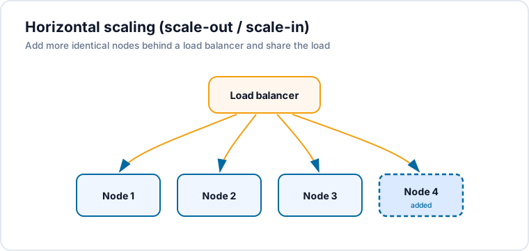
Horizontal scalability would instead buy more units of the same bus, rather than replacing the fleet. More vehicles on the route distribute passengers among themselves — exactly how horizontal scaling works: add or remove compute units (servers, containers, replicas). When a single-node web app starts receiving heavy traffic, you add replicas to split the load, usually behind a load balancer. When that capacity is automated, it’s called elasticity. For it to work well, the system needs a distributed architecture that can process requests with external parallelism. The matching operations are scale-out (add servers/replicas performing the same function) and scale-in (remove them) — combined to dynamically adjust capacity as demand oscillates.
Capacity and scalability planning
This is where it gets concrete. The base formula below is drawn from how Kubernetes’ Horizontal Pod Autoscaler (HPA) works, but it’s generic enough to apply in many contexts. The goal: figure out how many compute units a system needs to clear a bottleneck.
The base formula
The formula determines the ideal replica count to serve the system. In general terms, multiply the current number of replicas by the ratio between the metric’s current value and its desired value:
desiredReplicas = ceil( currentReplicas × (currentMetric / desiredMetric) )
The “desired value” is the target we want the metric to reach; the “current value” is what’s measured right now. It reads abstract until you plug in numbers — so let’s do that.
By resource utilisation (CPU / memory)
The simplest application uses CPU and memory utilisation — metrics easy to compute, plan, and monitor, which is why they’re so common in autoscaling. Excess utilisation signals a bottleneck, and the formula points at the adjustment.
Start from 6 replicas, each able to use 200 millicores, with 1200m requested against 600m available and a target of 80% utilisation. The intermediate step gives the current utilisation, then the base formula gives the replica count:
currentCPU%     = requested / available × 100 = 1200 / 600 × 100 = 200%
desiredReplicas = 6 × (200 / 80) = 15 replicas
To clear the CPU bottleneck, you’d scale from 6 to 15 replicas. The same logic applies to any resource, not just CPU.
By throughput (requests over time)
A favourite approach plans capacity from the number of requests the app receives in a period. The premise: each replica sustains a certain number of transactions per second without degrading. If each replica handles 10 TPS and the app receives 100 TPS, you’d want 10 replicas.
Start from 6 replicas, each sustaining 15 TPS, with 10,000 requests in the last minute. First the total throughput, then requests-per-replica, then the formula:
totalThroughput = 10000 / 60      ≈ 166.66 rps
perReplica      = 166.66 / 6      ≈ 27.78 rps
desiredReplicas = 6 × (27.78 / 15) ≈ 11 replicas
For a horizontal-scaling adjustment, 11 replicas would be the ideal target for this app.
Software scalability
Scalability goes far beyond elastic infrastructure. Tying it only to infra components is a mistake: looking at architecture, business needs, and flows while designing software is what lets you build modern solutions without inflating operating cost.
The first front is optimising algorithms in existing code — reducing computational complexity, eliminating processing bottlenecks, improving memory use, and exploiting parallelism and concurrency. At the data layer, optimising schemas, indexes, and queries lowers response time and expands capacity, as does distributing load across multiple servers. Other strategies include evaluating NoSQL or distributed storage for high demand, applying caching (in-memory, distributed, or client-side), and using queues and asynchronous messaging for intensive or I/O-bound tasks. Integrating these takes a continuous commitment to code quality, architecture, and monitoring — so the system evolves alongside its demands.
Key takeaways
- The three pillars reinforce each other. Performance sets the per-transaction limits; capacity plans around them; scalability moves them. Study one in isolation and you’ll mis-size the other two.
- Watch the Four Golden Signals — through percentiles. Saturation, traffic, response time, and error rate tell the health story, but averages lie. A 200 ms mean can hide a 1,000 ms p99.
- A resource can degrade before 100%. Don’t wait for saturation to hit the ceiling; find the utilisation point where your latency starts to bend and scale ahead of it.
- Your system is as fast as its weakest link. Backpressure means the slowest component caps end-to-end throughput — over-provisioning everything else just buys idle capacity.
- Right-size with a formula, not a guess.
desiredReplicas = currentReplicas × (currentMetric / desiredMetric)— the HPA logic — turns CPU or throughput readings into a concrete replica count. - Scalability is a software problem too. Algorithms, indexes, caching, and async messaging often buy more headroom than another server ever will.
References
- Site Reliability Engineering — Google (the SRE book)
- The Four Golden Signals of Monitoring — Sysdig
- How to Manage the 4 Golden Signals — Site24x7
- Horizontal Pod Autoscaling: Algorithm details — Kubernetes
- HorizontalPodAutoscaler Walkthrough — Kubernetes
- Kubernetes Instance Calculator — learnk8s
- Backpressure Explained: The Flow of Data Through Software — Jay Phelps
- Back pressure — Wikipedia
- Amdahl’s Law — Wikipedia
- Why Averages Suck and Percentiles Are Great — Dynatrace
- Percentiles Made Easy — AppDynamics
- Response Times and What to Make of Their Percentile Values — OmbuLabs
- Release It! Design and Deploy Production-Ready Software — Michael T. Nygard
- Stupid Simple Scalability — SUSE / Rancher